가상 쇼핑몰 데이터 프로젝트
import pandas as pd# 데이터프레임 읽어오기
retail = pd.read_csv("/content/drive/MyDrive/데이터분석/OnlineRetail.csv")
retail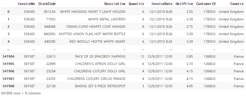
# 위 아래 데이터 3개씩 보이는 옵션
pd.options.display.max_rows = 6

retail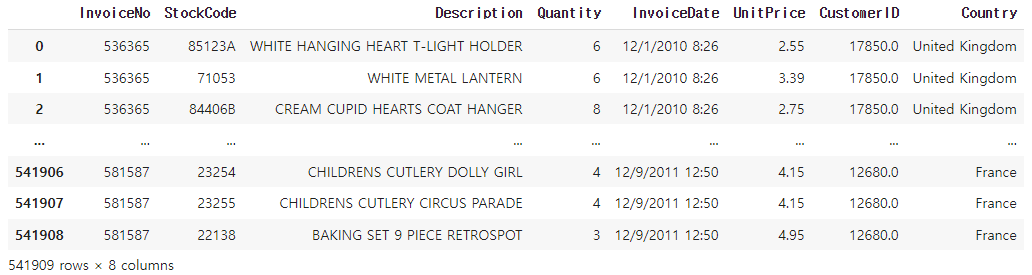
# info()로 간략한 정보 확인
retail.info()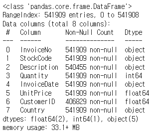
컬럼 설명
- invoiceNo : 주문번호
- StockCode : 상품코드
- Description : 상품설명
- Quantity : 주문수량
- InvoiceDate : 주문날짜
- UnitPrice : 상품가격
- CustomerID : 고객 아이디
- Country : 고객거주지역(국가)
# 각 필드당 null이 몇 개 있는지 확인
retail.isnull().sum()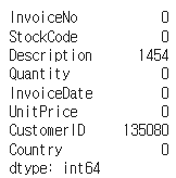
# 각 필드당 null이 몇 % 있는지 확인
retail.isnull().mean()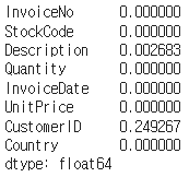
# 비회원 제거하기
retail = retail[pd.notnull(retail["CustomerID"])]

len(retail) # 406829
# 주문 수량이 0이하인 데이터 확인
retail[retail["Quantity"] <= 0]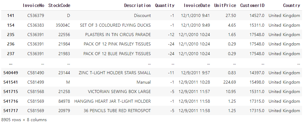
# 구입 가격이 0이하인 데이터 확인
retail[retail["UnitPrice"] <= 0]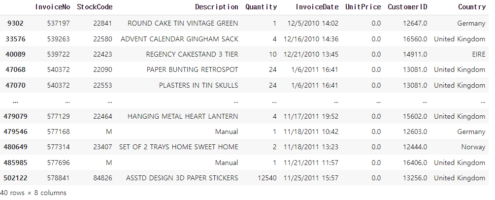
# 주문 수량이 1이상인 데이터 저장
retail = retail[retail["Quantity"] >= 1]
# 구입 가격이 1이상인 데이터 저장
retail = retail[retail["UnitPrice"] >= 1]

len(retail) # 304911
retail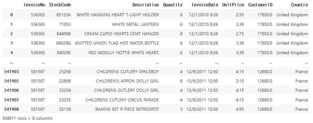
# 고객의 총 지출비용(CheckoutPrice) 파생변수 구하기
# 수량 * 가격
retail["CheckoutPrice"] = retail["UnitPrice"] * retail["Quantity"]
retail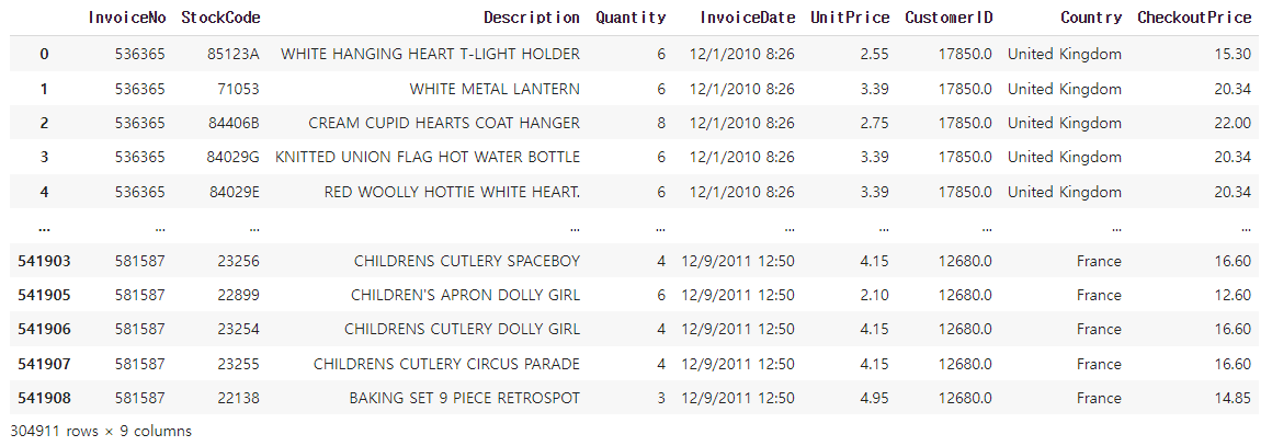
# 데이터프레임 info() 다시 확인
retail.info()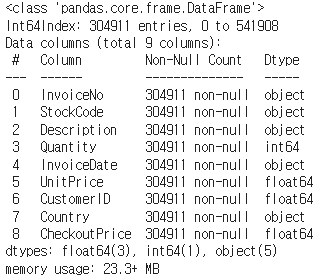
# head() 확인
retail.head()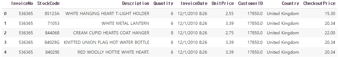
# 주문 날짜 컬럼 object -> datatime으로 바꿈
retail["InvoiceDate"] = pd.to_datetime(retail["InvoiceDate"])
# Dtype 확인
retail.info()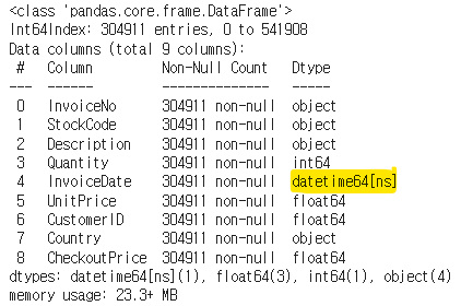
# 전체매출 구하기
total_revenue = retail["CheckoutPrice"].sum()
total_revenue # 7863916.5
# 몇 개국에서 주문했는지 계산
retail["Country"].value_counts()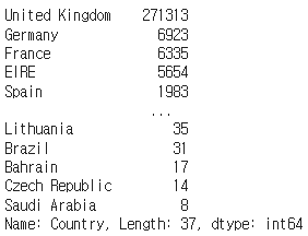
# 열 늘려주기
pd.options.display.max_rows = 40

# 다시 확인
retail["Country"].value_counts()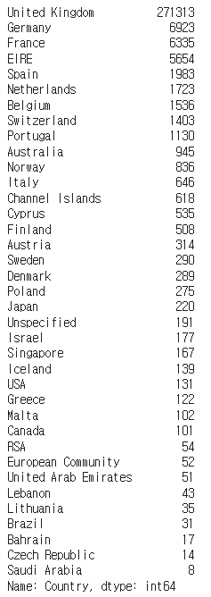
# 다시 원래대로 되돌리기
pd.options.display.max_rows = 10
# 국가별 매출 구하기
# 나라별로 그룹을 맺고, CheckoutPrice를 모두 더하고, 오름차순 정렬 시킴
rev_by_contries = retail.groupby("Country")["CheckoutPrice"].sum().sort_values()
rev_by_contries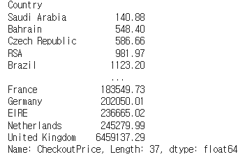
# plot 객체 생성
plot = rev_by_contries.plot(kind="bar", figsize=(20, 10)) # kind = "bar" 막대그래프
plot.set_xlabel("Country", fontsize=12)
plot.set_ylabel("Revenue", fontsize=12)
plot.set_title("Revenue By Contry", fontsize=15)
plot.set_xticklabels(labels=rev_by_contries.index, rotation=45) # 눈금을 나라이름으로 설정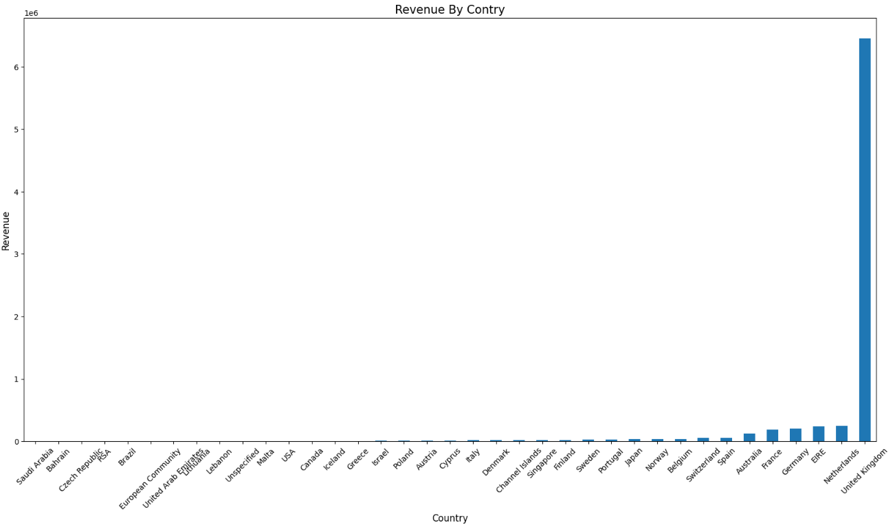
# 나라별 매출 % 구하기
rev_by_contries / total_revenue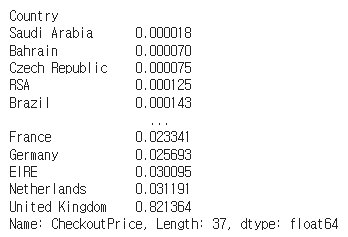
# 월별 매출 구하기
retail["InvoiceDate"].sort_values(ascending=False) # 날짜 내림차순 정렬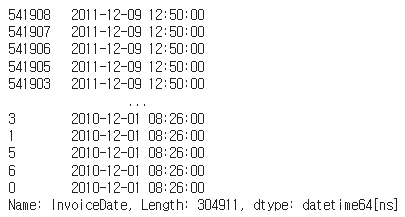
# 월별로 그룹 맺기 위한 함수

# 예) 2011-03-01 입력
def extract_month(date):
    month = str(date.month) # 3
    if date.month <10:
        month = "0" + month # 03
    return str(date.year) + month # 201103
# groupby 안에 익명함수나 콜백함수를 넣으면 모든 데이터에 대입하게됨
rev_by_month = retail.set_index("InvoiceDate").groupby(extract_month)["CheckoutPrice"].sum()
rev_by_month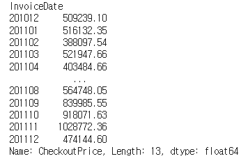
# plot 만들어주는 함수 선언
def plot_bar(df, xlabel, ylabel, title, rotation=45,titlesize=15,fontsize=12,figsize=(20,10)):
    plot = df.plot(kind="bar", figsize=figsize)
    plot.set_xlabel(xlabel, fontsize=fontsize)
    plot.set_ylabel(ylabel, fontsize=fontsize)
    plot.set_title(title, fontsize=titlesize)
    plot.set_xticklabels(labels=df.index, rotation=rotation)
# 월별 매출 그래프 그리기
plot_bar(rev_by_month, "Month", "Revenue", "rev by month")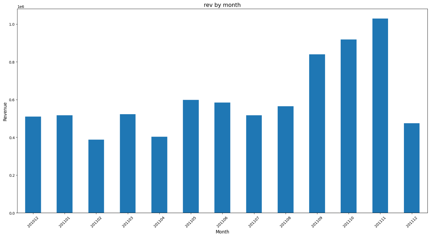
# 요일별로 그룹 맺기 위한 함수
def extract_dow(date):
    return date.dayofweek
rev_by_dow = retail.set_index("InvoiceDate").groupby(lambda date: date.dayofweek)["CheckoutPrice"].sum() # 람다 사용
rev_by_dow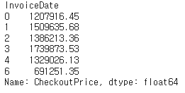
import numpy as np# 숫자로 되어있는 인덱스 번호를 문자로 변경
DAY_OF_WEEK = np.array(["Mon", "Tue", "Web", "Thur", "Fri", "Sat", "Sun"])
rev_by_dow.index = DAY_OF_WEEK[rev_by_dow.index]
rev_by_dow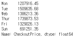
# 요일별 매출 그래프 그리기
plot_bar(rev_by_dow, "DOW", "Revenue", "Revenue By DOW")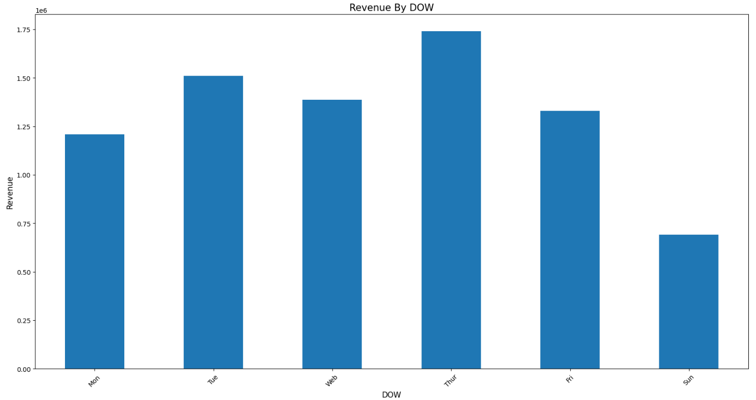
# 시간대별 매출 구하기
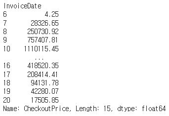
rev_by_hour = retail.set_index("InvoiceDate").groupby(lambda date: date.hour)["CheckoutPrice"].sum() # 람다 사용
rev_by_hour
# 시간대별 매출 그래프 그리기
plot_bar(rev_by_hour, "Hour", "Revenue", "Revenue By Hour")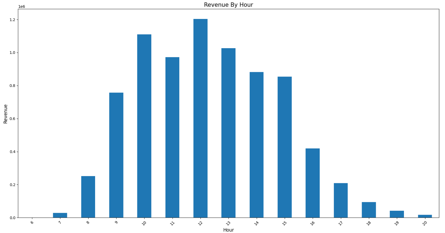
Quantity를 기준으로 판매제품(StockCode) Top 10 구하기
# 제품코드 확인
retail["StockCode"].info()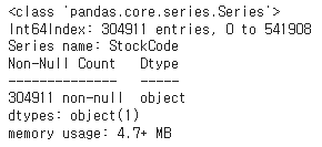
# StockCode로 그룹을 맺고, Quantity를 모두 더해, 내림차순 한 뒤, head(10)으로 상위 10개 데이터만 확인
stockCode_Top_10 = retail.set_index("StockCode").groupby("StockCode")["Quantity"].sum().sort_values(ascending=False).head(10)
stockCode_Top_10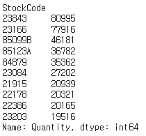
CheckoutPrice를 기준으로 우수 고객(CustomerID) Top 10 구하기
# CustomerID로 그룹을 맺고, CheckoutPrice를 모두 더해, 내림차순 한 뒤, head(10)으로 상위 10개 데이터만 확인
customerID_Top_10 = retail.set_index("CustomerID").groupby("CustomerID")["CheckoutPrice"].sum().sort_values(ascending=False).head(10)
customerID_Top_10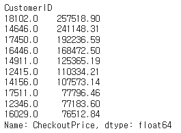
데이터로부터 lnsight
- 전체 매출의 약 82%가 UK에서 발생
- 11년도에 가장 많은 매출이 발생한 달은 11월
- 매출은 꾸준히 성장(11년 12월 데이터는 9일까지만 포함)
- 토요일은 영업을 하지 않음
- 새벽 6시에 오픈, 오후 9시에 마감이 예상
- 일주일 중 목요일까지는 성장세를 보이고, 이후 하락
'데이터 분석' 카테고리의 다른 글
| 7. 워드 클라우드(Word Cloud) (0) | 2023.06.13 |
|---|---|
| 6. 형태소 분석 (0) | 2023.06.12 |
| 4. 데이터프레임 활용하기 (0) | 2023.06.12 |
| 3. Matplotlib (1) | 2023.06.12 |
| 2-16. 원 핫 인코딩(One Hot Encoding) (1) | 2023.06.09 |


